The native secondary index is the less known and most misused feature of Cassandra.
In this article we’ll explain thoroughly the technical implementation of native secondary index
to highlight best use-cases and the worst anti-patterns.
For the remaining of this post Cassandra == Apache Cassandra™
A General architecture
Let’s say that we have the following users table:
 CREATE TABLE users(
     user_id bigint,
     firstname text,
     lastname text,
     ...
     country text,
     ...
     PRIMARY KEY(user_id)
 );
Such table structure only allows you to lookup user by user_id only. If we create a secondary index on the column country, the index would be a hidden table with the following structure
CREATE TABLE country_index(
    country text,
    user_id bigint,
    PRIMARY KEY((country), user_id)
);
The main difference with a normal Cassandra table is that the partition of country_index would not be distributed using the cluster-wide partitioner (e.g. Murmur3Partitioner by default).
Secondary index in Cassandra, unlike Materialized Views, is a distributed index. This means that the index itself is co-located with the source data on the same node. See an example below:
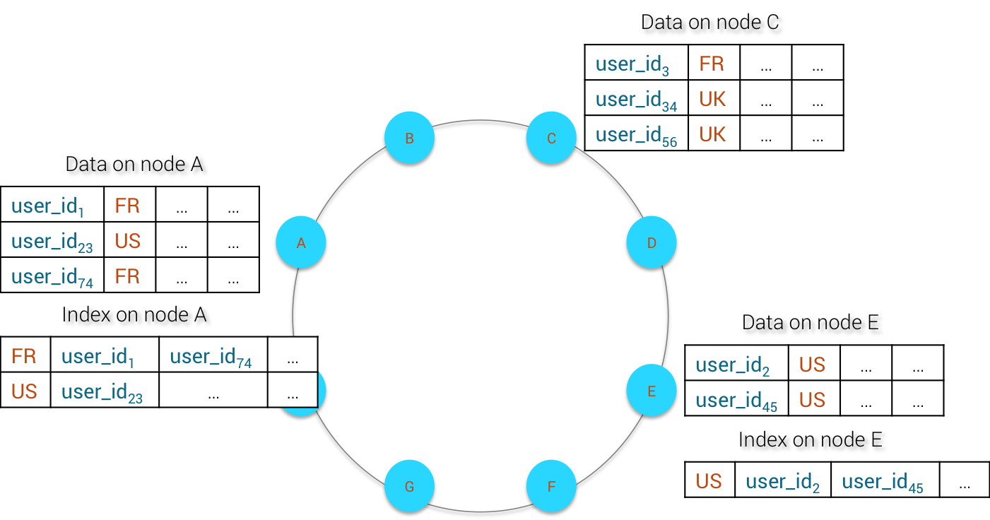
Distributed Index
The technical rationales to store index data along-side with original data are:
- reduce index update latency and the chance of lost index update
- avoid arbitrary wide partitions
Indeed if the index data has to be distributed across the cluster as normal data using the configured partitioner, we would face the same issue as with Materialized Views e.g. how to ensure that the index data has been written effectively to disk before acknowledging the mutation to the client.
A synchronous write of index data will definitely kill down the write latency and we’re not even considering Consistency Level into the game
By co-locating the index data on the same node as source data, a write to a table with index just costs an extra local mutation when flushing original data to SSTables (more details about it in the next chapter).
The second advantage of distributed index is to avoid arbitrary wide partitions. If we were to store in a single partition the country index, there will be 60 millions+ cells for the single FR country (assuming that we index all FR population). Imagine how wide the CN partition would be …
B Local write path
The write path to a table having native secondary index is exactly the same as for a normal table with respect to commit log. Whenever a mutation is applied to base table in memory (memtable), it is dispatched as notification to all registered indices on this table so that each index implementation can apply the necessary processing.
The native secondary index implementation just creates an inverted index for the hidden index table. It handles 3 types of operations:
- insert of new CQL row
- update of CQL row
- delete of CQL row
For scenario 1. the index just creates a new entry (partition key + clustering columns) into the index table.
For scenario 2. it is a little bit more involved. This scenario only occurs IF AND ONLY IF the new mutation is replacing a value that is still contained in the memtable. In this case, because Cassandra still has the previous value to be indexed, it will pass the previous and new value to the secondary index. The index manager will then remove the entry for the previous indexed value and add a new one for the new indexed value.
Scenario 3. is pretty straightforward, the secondary index just writes a tombstone to the index entry
Index memtable and base memtable will generally be flushed to SSTables at the same time but there is no strong guarantee on this behavior. Once flushed to disk, index data will have a different life-cycle than base data e.g. the index table may be compacted independently of base table compaction.
An interesting details to know is that the compaction strategy of the secondary index table inherits from the one chosen for the base table.
C Index data model
Now let’s look further in details how the schema for the inverse index is designed. Suppose we have a generic table
CREATE TABLE base_table(
    partition1 uuid,
    ...
    partitionN uuid,
    static_column text static,
    clustering1 uuid,
    ...
    clusteringM uuid,
    regular text,
    list_text list,
    set_text set,
    map_int_text map<int, text>,
    PRIMARY KEY((partition1, ..., partitionN), clustering1, ... , clusteringN)
);
1) Index on regular column
Suppose that we create an index on regular text column, the schema of the index table will be:
CREATE TABLE regular_idx(
    regular text,
    partitionColumns blob,
    clustering1 uuid,
    ...
    clusteringM uuid,
    PRIMARY KEY((regular), partitionColumns, clustering1, ..., clusteringM)
);
The partition key of regular_idx is the indexed value (regular) itself. The clustering columns are composed of:
- the base_table partition components collapsed into a single blob (partitionColumns)
- the base_table clustering columns
The idea here is to store the entire PRIMARY KEY of the CQL row containing the indexed regular value
2) Index on static column
Suppose that we create an index on static_column text column, the schema of the index table will be:
CREATE TABLE static_idx(
    static_column text,
    partitionColumns blob,
    clustering1 uuid,
    ...
    clusteringM uuid,
    PRIMARY KEY((regular), partitionColumns)
);
Indeed, since a static value is common for all CQL rows in the same partition, we only need to store a reference to the partition key of the base_table
3) Index on Partition component
If we create an index on the partitionK uuid component, the schema of the index table will be:
CREATE TABLE partition_idx(
    partitionK uuid,
    partitionColumns blob,
    clustering1 uuid,
    ...
    clusteringM uuid,
    PRIMARY KEY((partitionK), partitionColumns, clustering1, ..., clusteringM)
);
Strangely enough, instead of just storing the partitionColumns, Cassandra also stores the all the clustering columns of the base table.
The reason is that secondary index for static columns has been implemented recently. I have created a CASSANDRA-11538 to grant the same treatment for partition component index
4) Index on Clustering column
It is possible to have an index on the clustering column. Let’s suppose that we index clusteringJ uuid, 1 ≤ J ≤ M. The corresponding clustering index schema will be:
CREATE TABLE clustering_idx(
    partitionColumns uuid,
    partitionKeys blob,
    clustering1 uuid,
    ...
    clusteringI uuid,
    clusteringK uuid,
    ...
    clusteringM uuid,
    PRIMARY KEY((clusteringJ), partitionColumns, clustering1, clusteringI, clusteringK, ..., clusteringM)
);
Indeed, the index stores the clusteringJ as partition key, the complete partitionColumns as a single blob and the original clustering columns of the rows except clusteringJ because we have already its value as partition key
5) Index on list value
Let’s say we want to index values of list_text list<text>, Cassandra will create the following index table:
CREATE TABLE list_idx(
    list_value text,
    partitionKeys blob,
    clustering1 uuid,
    ...
    clusteringM uuid,
    list_position timeuuid,
    PRIMARY KEY((list_value), partitionColumns, clustering1, ..., clusteringM, list_position)
);
In addition of the complete primary key of the base table, the index table also stores the position of the indexed value within the list e.g. its cell name = list_position. This cell name has timeuuid type
5) Index on Set value
If we index the set_text set<text> column, the corresponding index table would be:
CREATE TABLE set_idx(
    set_value text,
    partitionKeys blob,
    clustering1 uuid,
    ...
    clusteringM uuid,
    set_value text,
    PRIMARY KEY((set_value), partitionColumns, clustering1, ..., clusteringM, set_value)
);
We store the complete primary key of the base table + the cell name of the set_text set, which happens to be the indexed value itself
6) Index on Map value
If we index the value of map_int_text map<int, text> column, the corresponding index table would be:
CREATE TABLE map_value_idx(
    map_value text,
    partitionKeys blob,
    clustering1 uuid,
    ...
    clusteringM uuid,
    map_key int,
    PRIMARY KEY((map_value), partitionColumns, clustering1, ..., clusteringM, map_key)
);
This time, the cell name of the map_int_text column is the map key itself.
7) Index on Map Key and Entry
If you index on map key, the index table would resemble:
CREATE TABLE map_value_idx(
    map_key int,
    partitionKeys blob,
    clustering1 uuid,
    ...
    clusteringM uuid,
    PRIMARY KEY((map_key), partitionColumns, clustering1, ..., clusteringM)
);
An index created on map entry (key/value) would create:
CREATE TABLE map_entry_idx(
    map_entry blob,
    partitionKeys blob,
    clustering1 uuid,
    ...
    clusteringM uuid,
    PRIMARY KEY((map_entry), partitionColumns, clustering1, ..., clusteringM)
);
The map_entry column is just a blob containing the key/value pair serialized together as byte[ ].
Please notice that for map key and map entry indices, the PRIMARY KEY of the index tables does not contain the map_key column as last clustering column, as opposed to map value index implementation.
D Local Read Path
The local read path for native secondary index is quite straightforward. First Cassandra reads the index table to retrieve the primary key of all matching rows and for each of them, it will read the original table to fetch out the data.
One naïve approach would be for each entry in the index table, request the data from the original table. This approach, although correct, is horribly inefficient. The current implementation groups the primary keys returned by the index by partition key and will scan the original table partition by partition to retrieve the source data.
E Cluster Read Path
Unlike many distributed search engines (ElasticSearch and Solr to name the few), Cassandra does not query all nodes in the cluster for secondary index searching. It has a special algorithm to optimize range query (and thus secondary index search query) on the cluster.
Querying all nodes (or all primary replicas) in on query to search for data suffers from many problems:
- on a large cluster (1000 nodes), querying all primary replicas (N/RF, N = number of nodes, RF = replication factor) is prohibitive in term of network bandwidth
- the coordinator will be overwhelmed quickly by the amount of returned data. Even if the client has specified a limit (ex: LIMIT 100), on a cluster of 100 nodes with RF=3, the coordinator will query in parallel 34 nodes, each returning 100 rows so we end up with 3400 rows on the coordinator JVM heap
To optimize the distributed search query, Cassandra implements a sophisticated algorithm to query data by range of partition keys (called Range Scan). This algorithm is not specific to secondary index but is common for all range scans.
The general idea of this algorithm is to query data by rounds. At each round Cassandra uses a CONCURRENCY_FACTOR which determines how many nodes need to be queried. If the first round does not return enough rows as requested by the client, a new round is started by increasing the CONCURRENCY_FACTOR.
Remark: Cassandra will query the nodes following the token range so there is no specific ordering to be expected from the returned results
Below is the exact algorithm:
- select first the index with the lowest estimate returned rows e.g. the most restrictive index. Cassandra will filter down the resulSet using the other indices (if there are multiple indices in the query).The estimate returned rows for a native secondary index is equal to the estimate of number of CQL rows in the index table(estimate_rows) because each CQL row in the index table points to a single primary key of the base table. This estimate rows count is available as a standard histogram computed for all tables (index table or normal one)

Estimated_rows_by_token_range
We use local data for this estimate based on the strong assumption that the data is distributed evenly on the cluster so that local data is representative of the data distribution on each node. If you have a bad data model where the data distribution is skewed, this estimate will be wrong.
- next, underestimate a little bit the previous estimate_rows_by_token_range value by multiplying it with a CONCURRENT_SUBREQUEST_MARGIN (default = 0.1) to increase the likelihood that we fetch enough CQL rows in the first round of query
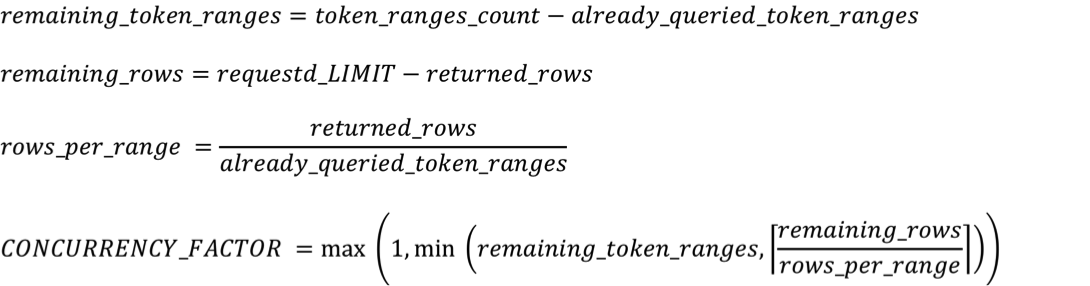
- determine the CONCURRENCY_FACTOR e.g. the number of nodes to contact for the current round of query. The formula is given by:

Concurrency-Factor-Formula
requested_LIMIT corresponds to the limit set by the query (`SELECT … WHERE … LIMIT xxx`) or by the query fetchSize when using server-side paging.
- then start querying as many nodes as CONCURRENCY_FACTOR
- if the first round rows count satisfies the requested_LIMIT, return the results
- else update the CONCURRENCY_FACTOR with the algorithm below and start another round of query
- if returned_rows = 0 then
CONCURRENCY_FACTOR = token_ranges_count – already_queries_token_ranges - else
Updated-Concurrency-Factor
- if returned_rows = 0 then
Below is an illustration of how it works on a 8 nodes cluster:
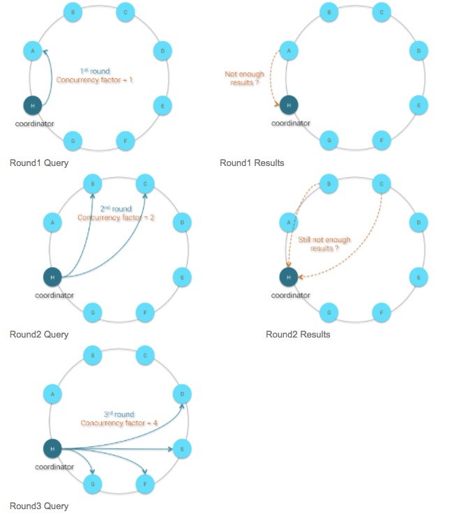
Range-Query-Cinematics
The curious reader can refer to the class `StorageProxy.RangeCommandIterator` and the method `StorageProxy::getRangeSlice()` for the source code of this algorithm.
F Best use case for native and other implementations of secondary index
Because of how it is implemented cluster-wide, all secondary index implementations work best when Cassandra can narrow down the number of nodes to query (e.g. narrow down the token ranges to query). This target can be achieved if the client query restricts the partition key:
- with a single value (`WHERE partition = xxx`). This is the most efficient way to use secondary index because the coordinator only needs to query 1 node (+ replicas depending on the requested consistency level)
- with a list of partition keys (`WHERE partition IN (aaa, bbb, ccc)`). This is still quite efficient because the number of nodes to be queried is bounded by the number of distinct values in the IN clause
- with a range of token (`WHERE token(partition) ≥ xxx AND token(partition) ≤ yyy`). This token range restriction avoids querying all primary replicas in the cluster. Of course, the narrower the token range restriction, the better it is
E Caveats
There are some well known anti-patterns to avoid when using native secondary index:
- avoid very low cardinality index e.g. index where the number of distinct values is very low. A good example is an index on the gender of an user. On each node, the whole user population will be distributed on only 2 different partitions for the index: MALE & FEMALE. If the number of users per node is very dense (e.g. millions) we’ll have very wide partitions for MALE & FEMALE index, which is bad
- avoid very high cardinality index. For example, indexing user by their email address is a very bad idea. Generally an email address is used by atmost 1 user. So there are as many distinct index values (email addresses) as there are users. When searching user by email, in the best case the coordinator will hit 1 node and find the user by chance. The worst case is when the coordinator hits all primary replicas without finding any answer (0 rows for querying N/RF nodes !)
- avoid indexing a column which is updated (or removed then created) frequently. By design the index data are stored in a Cassandra table and Cassandra data structure is designed for immutability. Indexing frequently updated data will increase write amplification (for the base table + for the index table)
If you need to index a column whose cardinality is a 1-to-1 relationship with the base row (for example an email address for an user), you can use Materialized Views instead. They can be seen as global index and guarantee that the query will be executed on only one node (+ replicas depending on consistency level).
Article originally published on www.planetcassandra.org
Don’t use with low cardinality, don’t use with high cardinality, so when i can use it? 😀
Thanks much for this article. Really appreciate the work you have put in explaining things at such length. Also thanks for pointing to the corresponding C* source code, that really helped to scratch the itch.
Thanks, tis is a super article. Now I’m going to read it again to see if I can understand it. 😉